Vertical partitioning
April 4, 2009For the past few weeks, I’ve been working on a Haskell program that give recommendations to developers in order to ease the process of vertical partitioning.
This program explores the code source of our web applications, and parses the PHP source code in order to list the different requests that are made on a given table.
This parsing process creates a list of Query objects, each Query representing the list of fields selected during a call to the ORM. This method has the obvious inconvenient to give equal weight to all the requests, but static analysis is the only thing available to me now; it would be better to weigh each query by the number of times it is called, but I do not have this information.
Lazy loading for easier coding 
During the parsing process, the module description files are loaded and fields are checked against the object definitions. With Haskell’s lazy evaluation, I wrote my code so that every single module would be loaded… but that’s not what actually happens: Haskell will only execute a small part of the code and only load the modules that I’m going to use. The other modules are really just closures to functions capable of reading a module definition; as long as they are not called, nothing happens.
Usually, only about 1% of all modules are opened and parsed.
Correlations between fields 
For all possible pairs of fields (n×(n-1)/2 pairs), a distance is computed using the simple Jaccard Index: this creates a complete graph with n vertices. This distance index indicates how often two fields are used together: two fields that are always selected together have a distance of zero, and two fields that are never together have a distance of one.
It seems like a lot of processing, but even for large table the number of edges stays acceptable: a 100-column table creates a graph with 100 vertices (if they’re all used in the code) and 4950 edges.
A filter then removes all the edges with distances above a certain threshold, and displays the graph using graphviz.
Since we’ve kept only the strongest links, we see clusters emerge. These clusters are groups of fields which are often used together in the code, but don’t tend to be used with anything else. If in a group of fields that are often seen together there exists no other strong link to another field, it can be a candidate for extraction in a separate table. An engineer will not use this directly, but use it as advice.
Example 
Consider this code, written using our PHP framework:
// get the 5 oldest of this area.
$this->mPerson
    ->select('id', 'name')
    ->getGroup(0, 5);

$this->mPerson
    ->select('father', 'mother', 'birth')
    ->getGroup();

$this->mPerson
    ->select('country', 'city', 'postcode')
    ->getGroup();
This graph is produced: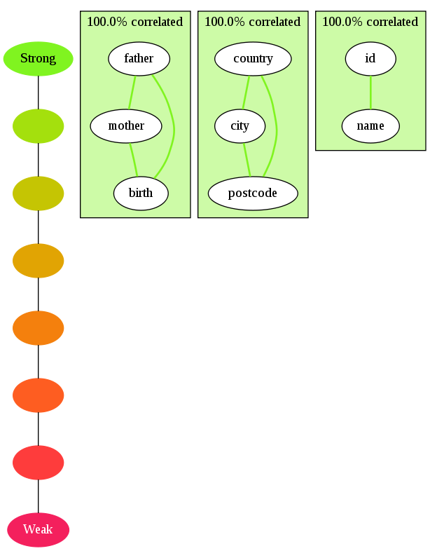
Indeed, these fields are always selected together, and are never mixed with anything else.
Now, if we add these two calls:
$this->mPerson
    ->select('id', 'name', 'age')
    ->getGroup();

$this->mPerson
    ->select('id', 'name', 'sex')
    ->getGroup();
The last block changes as such: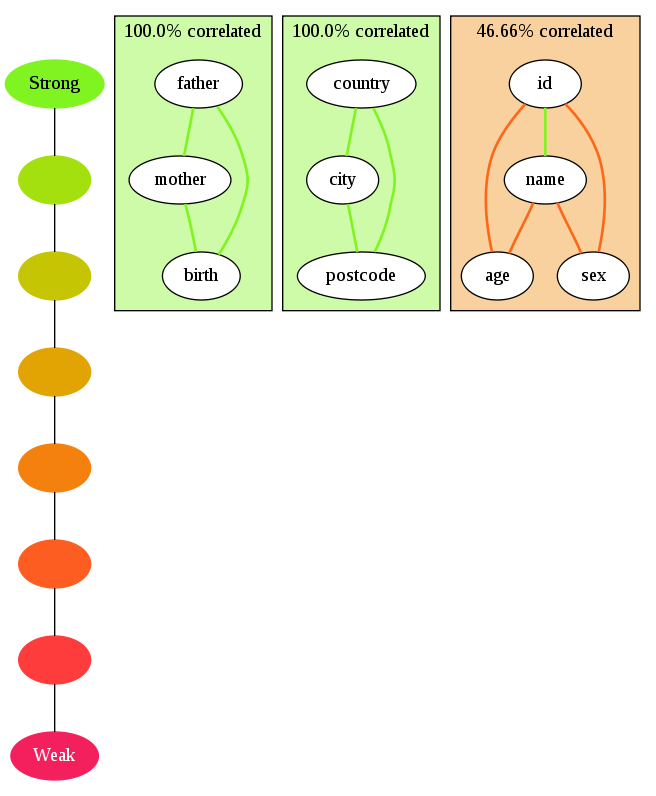
Adding these lines adds the age and sex fields and links them to id and name. There is a strong correlation between the presence of id and the presence of name, and this is shown by the green color of their common edge (the other links are weaker). The cluster’s background color shows that the internal consistency of this group is quite low.
Tweaking 
This tool does not give ready-made database schemas, but only shows the dependencies between columns. The engineer using this program changes the distance threshold to get different dependencies: the highest the threshold, the weaker the clusters. Raising it can lead to important discoveries: for instance, it can help detect an important link between a strong core of fields and a seldom-used but important field that might get cut by a low threshold. In that case, cutting out this core without realising which hidden dependencies might be affected would be a serious mistake.
Performance 
As I mentioned earlier, laziness made it easy to write readable code while getting some performance for free. I’ve also used the Parsec library to parse the ORM calls; its elegance and speed make it a remarkable tool.
The bottleneck is often graphviz’s “dot” program, which can take a while to draw a few dozen nodes with hundreds of edges. This program was not profiled or optimized for speed, as it needs only a few seconds to analyse our 200,000 lines of code.
Real-world overview 
This is the output of the program with default options on our largest table, which has 85 columns.
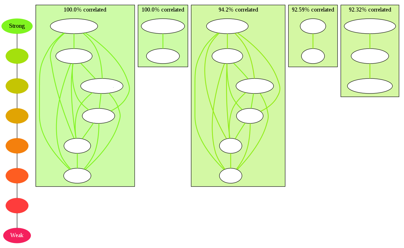
I apologize for the lack of field names, but I don’t think it would be appropriate for me to publish this kind of information.
After the default run, most of the fields have been completely cut out, by lack of strong links attached to them. This default run shows an interesting pattern, with two clusters organized in exactly the same way. This is a good example of an organic growth, where field modifiers have been added and are used like the fields they depend on; think of a Character table with skills a,b,c,d and bonuses applied to these skills by creating aBonus, bBonus… all added after the skills, in the same table. These 2 clusters would be {a, b, c, d} and {aBonus, bBonus, cBonus, dBonus}.
An option is used to bring back fields that have been cut out, by showing each field’s strongest link even if it is under the threshold:
The color progression shows that the last groups have a very low score, which means that there are a lot of hidden links attached to these nodes. Still, keeping the strongest link for the “saved” ones helps maintain some meaning: even the last group is made of fields which actually go together!
But there is a downside to this technique: a few rare fields are attached to strong clusters via a weak link (their strongest). This can sometimes lower the quality of otherwise good clusters, and this is the case here in the second and third clusters. In order to be able to view lonely fields while still retaining uncontaminated clusters, an command-line option enables the creation of a “lonely pool”, where fields with no link left are displayed without any structure.
Displaying the rest of the fields while tweaking the cluster threshold is useful reminder that moving columns out can be a big deal, even if the table seems small when most of its columns are hidden.
It is the role of the engineer doing the partitioning to examine different thresholds, as there is currently no way to select a “best” value. Is there even one?
This is what the table looks like at with different values:
Cut at 0.1: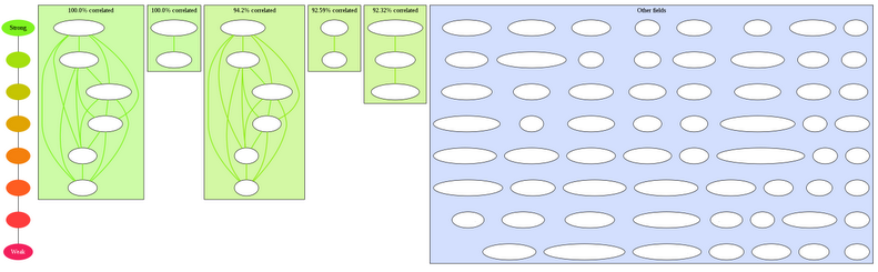
Cut at 0.2: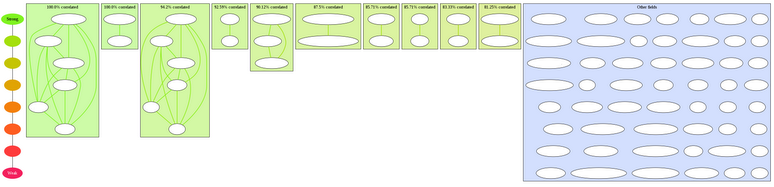
Cut at 0.4: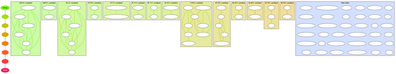
Last points 
In my opinion, the data should not come from the source code, but from the database log. Some queries are run hundreds of times more often than others, and such a naïve source code analysis misses this very important point.
Several improvements are planned, such as the ability to ignore such and such fields or to evaluate the complexity of an extraction by counting the number of calls that will need to be changed.
Haskell was the perfect tool here. The mathematical constructions used to compute the correlations are expressive and readable. The purity of the language surely avoided many common mistakes.